Measuring Headways
The following document outlines the simple process of using a smart phone to record headways at an intersection and to study headway distributions and the concept of lost times from the recorded data. The data recording process is very straight forward, as explained below, and can easily be followed using any modern smart phone camera. Free video playback / editing software can be used to extract meaningful data visually from the video recording to obtain the headways of various vehicles.
These instructions can be used as a teaching project for Transportation Engineering under-graduate classes where students get a chance to record and observe the basic intersection signal design concept of lost time and headway distribution.
We would greatly appreciate if you share your experience and your data (average headways, and observation location) with us if you do use this project yourself.
List of Topics
Instructions
1. Picking a location
You first need to pick an intersection and a time for the study. Pick a location that allows you to stand and record video of the intersection safely (preferably from a side-walk), without any major obstacles (such as trees) obstructing your view of the intersection. The time you pick should allow you to record the traffic and the signal well enough such that you are able to observe clearly as vehicles move, and you can also see the signal changing from red to yellow to green.Another important requirement is the presence of high demand at the location. This study is only useful if start-up times of at least 7 or 8 vehicles can be noted. Thus, one should pick a location where a queue of 7 or more vehicles forms consistently during each red phase. (Note: it is ok to have a few cycles with smaller queues, and the observed cycles also do not need to be consecutive cycles).
- Should be able to record safely
- Should be able to record the signals changing
- Should be able to see vehicles as they cross stop line
- Watch out for obstructions to view such as poles, trees etc.
- Observe traffic for a while. Avoid locations where vehicles on other lanes might be obstructing view of vehicles on lane on interest. This might make data extraction complicated later. You might need to either adjust position or recording angle to overcome complications, or choose a different location / lane to observe.
- Location should have at least 6-7 vehicles queueing per lane
2. Setting up the camera
As mentioned earlier, it is important to set up the camera in such a way that both the traffic signal as well as the stop line on the direction of interest are clearly visible. From the video, we will want to extract the exact time when the signal turns green, as well as exact times when vehicles cross the stop line. The figure below illustrates what a good coverage / view set-up would be. In the figure, the traffic signal can be clearly seen towards the right top corner, and the yellow stop line is also visible roughly around the center of the video screen.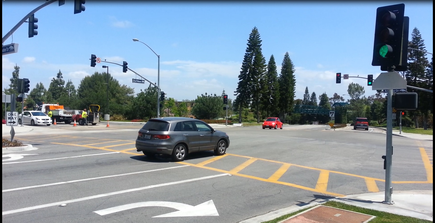
- Make sure that the recording angle is good by taking pictures and making sure the signal and the stop line are clearly visible.
- Should be able to record the signals changing
3. Getting ready to record
With the orientation of the camera adjusted so that all required details are observable, the recording process itself can be started. Using a tripod to ensure stable recording is recommended, but is not necessarily required. If not using a tripod, try to make sure the video is not too jerky, and that all features are always covered in the video (such as the signal falling out of the video frame). Before recording each cycle, you will also need to make a note of the number of vehicles in the queue prior to green.- Prepare to record over multiple cycles (5-10).
- Cycles should have queued vehicles at start of green phase.
- Prepare to note the number of queued vehicles for each recorded cycle (either take a picture of of the vehicles before green, or call out the number so that it can be heard in the video). This is needed later since only queued vehicles can be used for headway analysis.
4. Recording over multiple cycles
The headway pattern of vehicles is typically studied at an aggregation level. This is done in order to eliminate the variability due to driving behaviours and statistical errors. Thus, typically, one would want to record data over multiple cycles (the higher the better, but patterns start becoming visible with as few as 5-10 cycles). The average headways can then be extracted for each queue position.You should record a video (or multiple videos) that covers at least 5 signal cycles (5 different instances of the signal switching from red to green) with each having at least 6 vehicles queued. During the recording phase, also make a note of how many vehicles are in the queue, stopped, at the instance that the signal turns green. Any vehicle that is not a part of the completely stopped queue, would have a smaller headway and lower lost time due to not having to start from 0 zero. Such vehicles should be filtered out (vehicles rolling at close to 0 speed need not be eliminated).
- Record at least 5 complete signal cycles.
- The cycles you would be using for analysis should have at least 6 vehicles queued each.
- Make a note of number of queued vehicles at start of green for each cycle. Vehicles not queued should be filtered out of observations.
5. Processing the Video
Once the video(s) have been recorded, the data needs to be processed. The key elements to note, are the times at which the signal changed to green from red, and the times at which the queued vehicles crossed the stop line. Various video editing / playback tools allow playing back the video frame-by-frame in order to extract the above details. Avidemux is one such tool that is free to use.Using such a tool, you should note down the exact time instant (or frame) when:
- The signal switches to green first from a red phase; and
- A vehicle crosses the stop line.
 |
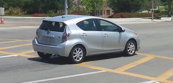 |
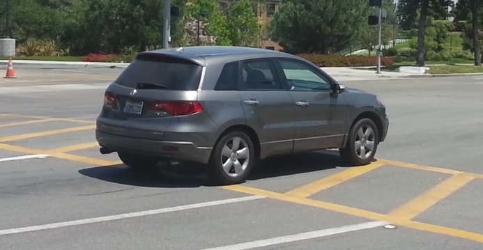
| Sample frames when vehicle rear wheels cross the stop line | |
The final observations should look something like the following:
| Cycle Number | 1 | 2 | 3 | 4 | 5 |
|---|---|---|---|---|---|
| Start of Green | 18.43 | 4.30 | 0.04 | 11.56 | 3.2 |
| 1st Veh. crossing | 22.46 | 8.44 | 3.94 | 15.96 | 6.9 |
| 2nd Veh. crossing | 25.39 | 11.20 | 6.81 | 19.00 | 9.6 |
| 3rd Veh. crossing | 28.09 | 13.90 | 9.14 | 21.89 | 11.8 |
| 4th Veh. crossing | 30.23 | 16.21 | 10.90 | 23.70 | 13.7 |
| 5th Veh. crossing | - | 18.03 | 12.84 | 26.23 | 15.6 |
| 6th Veh. crossing | - | 20.63 | 14.61 | 27.26 | 17.8 |
| 7th Veh. crossing | - | 22.20 | 16.30 | - | 19.8 |
Note: You can also note down other observations that you might find interesting to study, such as the time at which you first see the leading vehicle start moving, corresponding to the drivers' reaction time to the change in signal.
6. Extracting headways and calculating lost times
With the start of green, and stop-line crossing times of all vehicles noted, the headways for each vehicle can be easily extracted. The headway for the first vehicle is the time difference from the start of green to the vehicle crossing the stop line. The headway for all subsequent vehicles is the difference between the crossing time of that vehicle and that of the vehicle before it.Once the headways are extracted for each cycle, the average headway for each queue position can be calculated and plotted in a headway vs. queue position graph.
|
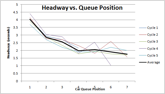 | |||||||||||||||||||||||||||||||||||||||||||||||||||||||||||||||
| Headway vs. Queue position table and corresponding graph based on sample data as shown earlier. | ||||||||||||||||||||||||||||||||||||||||||||||||||||||||||||||||
Finally, the start-up lost time of vehicles can be calculated from the headways. First identify the queue position 'm' past which the headway seems to saturate to roughly constant values (typically the 4th or 5th queue position). The expected saturation headway is then obtained as the average headway for all queue positions greater than 'm'. This saturation headway corresponds to the capacity flow-rate at the location. The difference between the observed headways of the initial vehicles (queue positions up to 'm') and the saturation headway gives that vehicle's lost time. The sum of lost times of all vehicles in queue gives the total start-up lost time.
Saturation Headway = hs = (1.98 + 2.05 + 1.90 + 1.75) / 4 = 1.92 secs
Total Start-up Lost Time = Σ(hi - hs) = (4.03 - 1.92) + (2.86 - 1.92) + (2.56 - 1.92) = 3.69 secs
Sample Worksheet for Calculating Headways
| Cycle Number | 1 | 2 | 3 | 4 | 5 |
|---|---|---|---|---|---|
| Start of Green | |||||
| 1st Veh. crossing | |||||
| 2nd Veh. crossing | |||||
| 3rd Veh. crossing | |||||
| 4th Veh. crossing | |||||
| 5th Veh. crossing | |||||
| 6th Veh. crossing | |||||
| 7th Veh. crossing |
| Cycle Number | 1 | 2 | 3 | 4 | 5 | Avg. |
|---|---|---|---|---|---|---|
| Headway | ||||||
| 1st Veh. | ||||||
| 2nd Veh. | ||||||
| 3rd Veh. | ||||||
| 4th Veh. | ||||||
| 5th Veh. | ||||||
| 6th Veh. | ||||||
| 7th Veh. |
Sample Recordings and Data
| Download Sample Video 1 |
Extracted Info | |
| Download Sample Video 2 |
Extracted Info | |
| Download Sample Video 3 |
Extracted Info | |
| Download Sample Video 4 |
Extracted Info | |
| Download Sample Video 5 |
Extracted Info |
Additional studies
Although the above project is to allow students to get a hands-on experience of recording traffic data, while also observing the exponentially decreasing headways and the corresponding concept of lost time, the study can easily also be extended in multiple ways. The following are a couple of suggestions for possible extension studies.Calibrating a Cell Transmission Model for queue discharge
Srivastava, Jin, and Lebacque (2014)[1] present a modified Cell Transmission Model that can capture vehicle discharge properties accurately at signalized intersections. This modified CTM updates Daganzo's original model through a new demand function. In doing so, the model is able to capture realistic queue discharge features such as discharge headways and discharge flow-rate. The paper also shows how the model may be calibrated against observed headways at an intersection. Thus, the data collected above, can be used directly to calibrate the modified CTM.Once the headway data has been collected, it is converted back to the corresponding passing times of vehicles assuming t=0 as the time at which the signal changed to green. Thus, the passing time t(i) is simply the sum of headways for vehicles 1 through i. Once t(i) is known for each queue position i, (and thus the inverse relation t(i) → i is also known), the model can be calibrated by minimizing the SSE between observed i and model obtained Â(t) by changing the model parameters, as shown below.
Â(t) = qct - L(qc/qj - 1)(kj - kc)(1-e-qjt/L(kj-kc)).
minimize ∑(Â(t) - i)2
Any non-linear optimization technique (such as the Nelder Mead method) can be used for the process. Further, if traffic features and parameters such as posted speed limit, and expected jam density, are known for the location, their values can either be fixed in the optimization set-up, or a feasible range be applied to them through appropriate constraints. For full details and a detailed explanation of the calibration process, refer to the original paper.
Reference:
[1] Srivastava, A., Jin, W.-L., Lebacque, J.-P., 2014. A modified cell transmission model for signalized intersections. In: Transportation Research Board 93rd Annual Meeting. No. 14-4713.
Study of traffic behaviour across multiple locations
One obvious extension of the above experiment, would be to record the headways across multiple locations, and see how similar / different the results are. If one finds observable differences, the next step would of course be to try and understand what the reasons for the differences are, and if it is possible to predict the headways at an unknown location.In picking multiple locations, either locations along the same corridor, locations with similar posted speed limits, or random independent locations might be picked. Picking locations in CBDs and comparing them with locations in suburbs and in residential areas might also offer interesting insights.
The study can similarly be repeated on a single location, but comparing across different lanes and/or approaches.
Study on reaction time of vehicles
Typically drivers take a finite amount of time to react to changes in their surroundings. Thus, there might be a lag between a signal changing to green, and the first vehicle to start accelerating as a consequence, or between a vehicle in front hitting its brakes, and the following vehicle hitting the brakes in reaction to it. The reaction time typically depends on the alertness and the response of the driver, including the time it takes for the observer to understand the situation, process the information in the brain, and for the response signal to be transmitted from the brain to say, the feet to change the pressure on the gas pedal or the brakes.The data recording above, can also be used to study certain aspects of reaction time. From the video, one can extract the times at which the first queued vehicle shows first signs of movement.
The reaction time for the changing signal would then be the difference in the time stamps of the signal changing to green, and the above mentioned time when the vehicle starts moving.
While observing the reaction time of first queued vehicle over multiple cycles through its mean and variance itself would be an interesting study (to compare against commonly accepted values), possible extensions could be to study whether the mean or the variance changes with the time of the day, weather conditions, type of vehicle, or location.